Stochastic Loading of Microfluidic Droplets
Droplet-based microfluidics are emerging as a useful technology in various fields of biomedicine. Both droplet digital PCR and droplet based culture methods require that droplets are created with either a single DNA molecule or a single cell per droplet. Obviously it is difficult to individually place DNA molecules or cells into droplets, instead people turn to stochastic models to estimate the distribution of cells per droplet, tuning the experimental parameters to achieve an acceptable distribution.
I felt uncomfortable by the Poisson approximation that I heard some people talk about and I wanted to derive a model myself. In full disclosure, I think that I was wrong, the Poisson is a good approximation for this setting but I needed to convince myself and derive the approximation. In this post I derive a Poisson approximation to this process and demonstrate how to calculate quantities of interest under uncertainty in lab measurements.
The Basic Model
The First Step - Multinomial
What made the most sense to me was to look at this as a Multinomial process with \(n\) total “units” (cells, DNA molecules, etc… ) and \(k\) categories (droplets). In using the multinomial in this way, I am assuming that each unit gets assigned to a droplet independent of the other units. In addition, I will assume a given unit has an equal probability of ending up in any given droplet.
Let \(\mathbf{x} = (x_1, \dots, x_k)\) represent the number of units assigned to each of \(k\) droplets. Note we know that \(\sum_i x_i = n\). We say that \[ \mathbf{x} \sim \text{Multinomial}(n, \mathbf{p}) \] where \(\mathbf{p} = (p_1, \dots, p_k)\) and \(p_i\) represents the probability that a unit will end up in droplet \(i\). We therefore also know that \(\sum_i p_i = 1\).
Focusing on our Question - Binomial
We are primarily interested in the distribution of the number of units that end up in given droplet. That is, we are interested in the marginal probability \(p(x_i = j)\) for \(j\in\{0, 1, \dots, n\}\). The marginal distribution turns out to be a Binomial Distribution with density
\[ p(x_i = j) = {n \choose j}p_i^j(1-p_i)^{n-j}, \quad j\in\{0, 1, \dots, n\}\].
This result comes from the helpful people at the University of Alabama in Huntsville Statistics Department (I love their site). However, as they point out, its actually really intuitive to derive (see their proof under section 2.). Essentially for a given droplet there is a certain probability that a given unit will end up in that droplet \(p_i\) and a certain probability that it will end up in any other droplet \(1-p_i\).
Approximating the Binomial - Poisson
The Binomial can be approximated by the Poisson when \(n \rightarrow \infty\) and \(p_i \rightarrow 0\) . In this case the Poisson approximation is given by \(np = \lambda\) where \(\lambda\) is the Poisson rate parameter.
When is the Poisson approximation to the Binomial valid?
This approximation really rests on \(n\) being “very large” and \(p\) being “very small”. So lets look at some values of \(n\) and \(p\) and see how the approximation fares.
library(tidyverse)
set.seed(4)

k <- c(2, 5, 10, 20, 200, 2000) # Various numbers of droplets
n <-  c(100, 500, 1000)         # Various numbers of units or cells to place in droplets
params <- expand.grid(n = n, k = k, j = 1:50) # look at combinations of these parameters

# The next two lines are just to make the labels in the plot look nice
n.labels <- paste("n =", n)
p.labels <- paste("p =", signif(1/k, 1))

params %>%
  mutate(p = 1/k,
         lambda.approx = n*p,
         j = j + floor(lambda.approx) - floor(mean(j)), # Explore near the mean of the distribution
         n.label = paste("n =", n),                        # Make plot look nice
         p.label = paste("p =", signif(p,1))) %>%          # Make plot look nice
  mutate(n.label = factor(n.label, levels = n.labels),     # Make plot look nice
         p.label = factor(p.label, levels = p.labels)) %>% # Make plot look nice
  filter(j >= 0) %>%                               # Only keep positive counts
  mutate(Binomial = choose(n, j)*p^j*(1-p)^(n-j),  # **The Distributions**
         Poisson = dpois(j, n*p)) %>%              # **The Distributions**
  ggplot(aes(x = j)) +                             # Everything else is just plotting
  geom_line(aes(y = Poisson)) +
  geom_point(aes(y = Binomial), shape = "o") +
  facet_wrap(n.label ~p.label , scales="free", nrow=3, ncol=6)+
  theme_bw() +
  ggtitle("Poisson Approximation vs. Binomial Distribution",
          "Poisson given by Black Line, Binomial by Open Circles")+
  ylab("Density")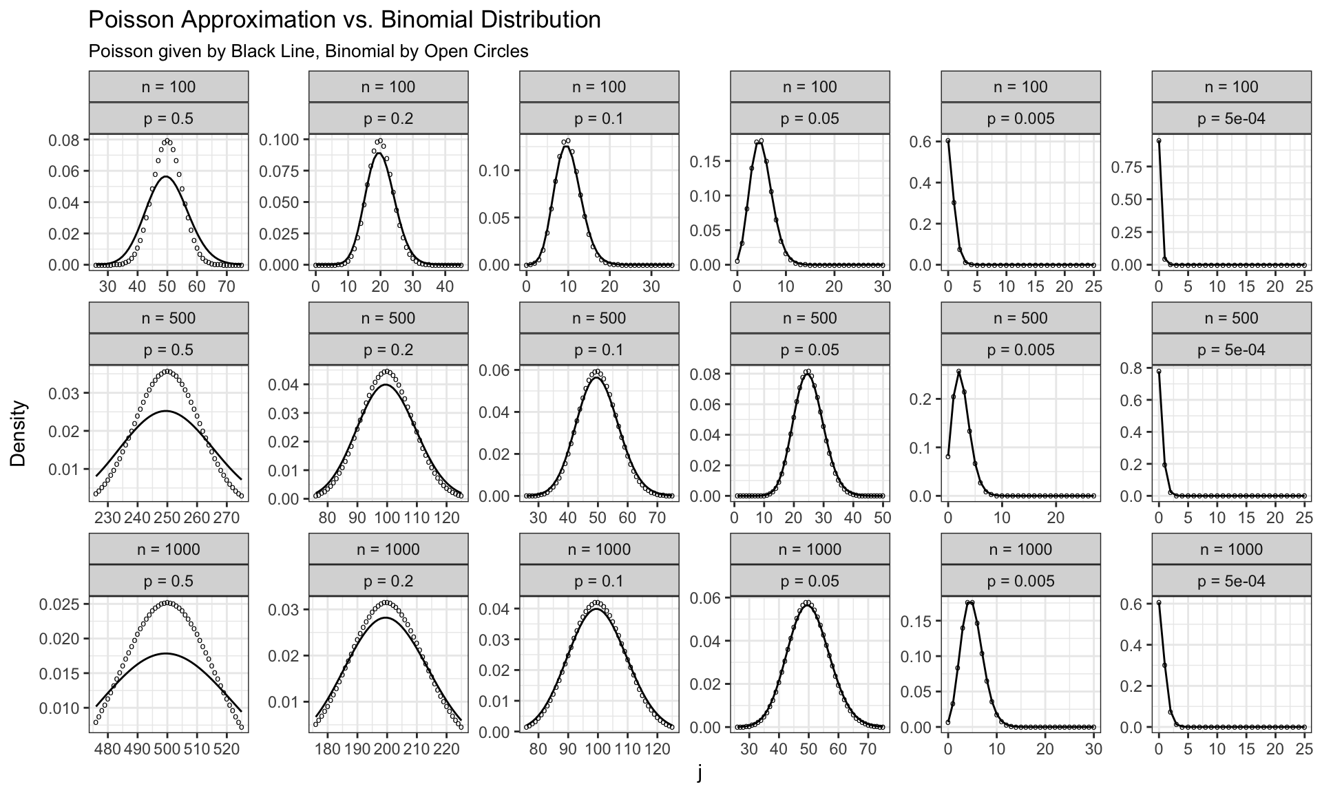
We see that for small \(n\) and large \(p\) (for example with \(n=100\) and \(p=0.5\)) the approximation is not great. However really for all parameters settings to the right of the second column in the above plot, the approximation seems appropriate.
Looking at Real Parameters Values
From the above results we know that for large \(n\) and small \(p\) we can approximate the binomial distribution with the Poisson as \(\lambda = np\) where \(\lambda\) is the Poisson rate parameter.
However, a few of my colleagues that are doing work with microfluidic droplets don’t measure the number of droplets directly, instead they measure the droplet diameter. With some dimensional analysis we can still calculate \(\lambda\). Note that the dimension of \(n\) was cells and the dimension of p was \(1/\)droplets; therefore we can write
\[lambda = np = \frac{cells}{droplets} = \frac{cells}{volume}\frac{volume}{droplets}.\] Thus we can calculate \(\lambda = np\) if we know the concentration of cells and the volume of each droplet. My colleague gave me the diameter of each droplet and we will assume that they are perfect spheres.
cells.per.ml <- 1e+06 # cells / mL
droplet.diameter <- 80 # microns
droplet.volume <- (4/3)*pi*((droplet.diameter/2)^3)*1e-12 # mL/droplet
lambda = cells.per.ml * droplet.volume
To figure out if we are in the big \(n\) small \(p\) regime lets assume we make 5mL of droplets.
ml <- 5
(n <- cells.per.ml * ml)
## [1] 5e+06droplets <- ml/droplet.volume
(p <- 1/droplets)## [1] 5.361651e-08So it does look like we are in the range where the Poisson approximation is valid. Lets now plot the Poisson approximation.
j <- 0:20
d <- data.frame(j = j, Poisson = dpois(j, lambda))
d %>%
  ggplot(aes(x=j, y = Poisson)) +
  geom_line() +
  theme_bw() +
  ylab("Density")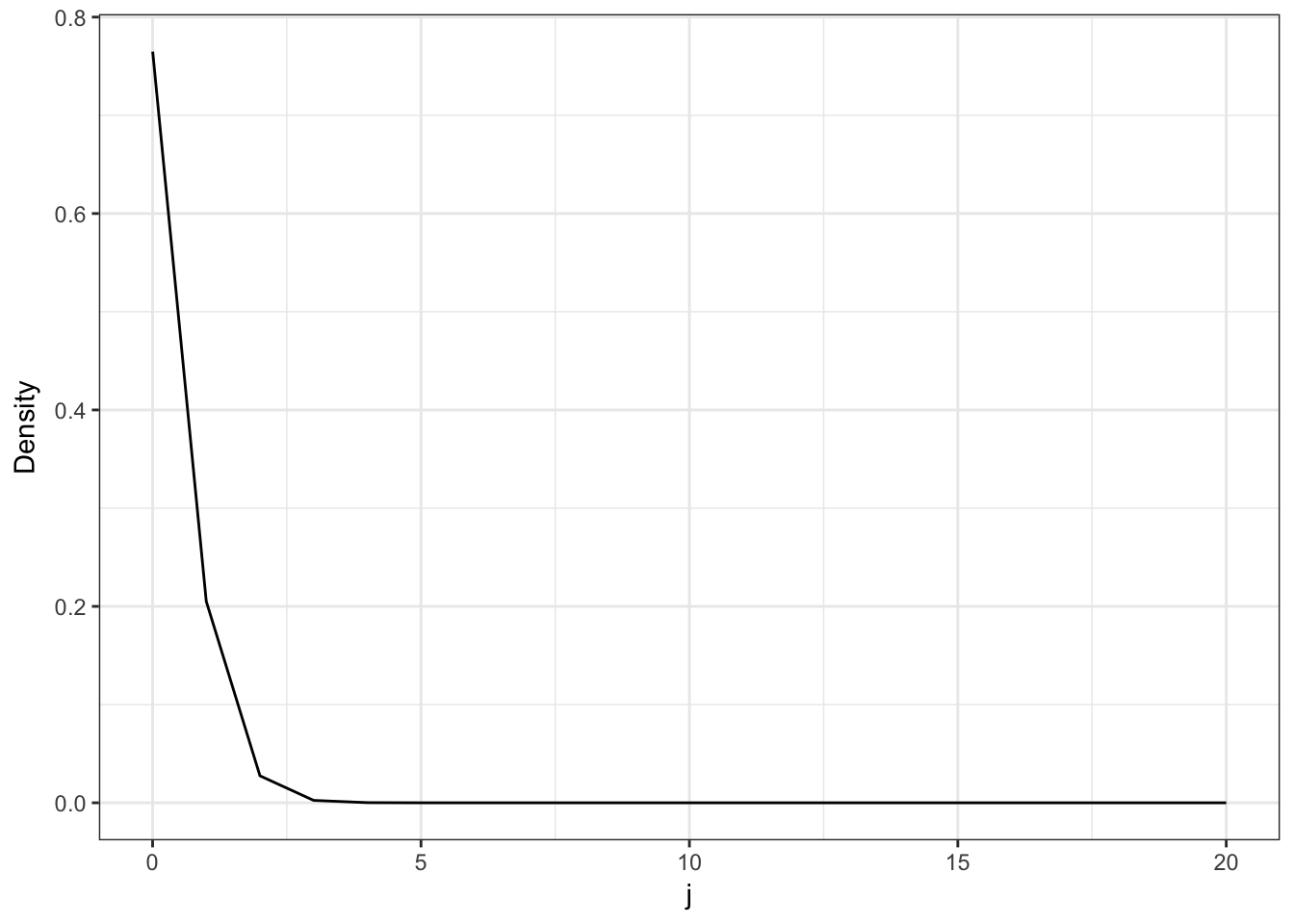
Now lets look at the ratio \(p(x_i=1)/p(x_i<1)\) which (for a large number of droplets) represents the ratio of droplets with only 1 cell each to the number of droplets with more than 1 cell each.
ratio <- d$Poisson[2]/(1-sum(d$Poisson[c(1,2)]))This ratio tells us that for every droplet with more than 1 cell in it there are approximately 6.8 droplets with only 1 cell in them.
Calculating the distribution of quantities in light of uncertainty in lab measurements
It turns out that it is actually quite difficult to calculate the concentration of certain cellular mixtures (especially with mixed microbial communities) and often there is some uncertainty with respect to the cells.per.ml parameter we set in the last section. Now I am just going to briefly demonstrate how we can simulate the distribution with the addition of this uncertainty.
I am going to assume that our uncertainty in the quantity cells.per.ml follows a normal distribution but almost any univariate distribution could be substituted here. A log normal distribution may be a better assumption if you think that the uncertainty exists on a log-scale (i.e., if you want the uncertainty to be in terms of fold-changes on a mean value). Note that I am actually using a truncated normal because I throw away the few samples where cells.per.ml is negative.
cells.per.ml <-  rnorm(1000, 1.6e6, sd = 5e5) # Concentration of cells
cells.per.ml <- cells.per.ml[cells.per.ml > 0] # truncation
droplet.diameter <- 80 # microns
droplet.volume <- (4/3)*pi*((droplet.diameter/2)^3)*1e-12 # mL/droplet
lambda = cells.per.ml * droplet.volume

j <- 0:20
d <- rep(0, length(lambda))  # Container to store results of for loop
for (i in 1:length(lambda)){ # For each of our sampled values
  x <- dpois(j, lambda[i])
  d[i] <- x[2]/(1-sum(x[c(1,2)]))
}
Before looking at the distribution of this ratio. Lets first look at our chosen distribution over possible values of cells.per.ml.
qplot(cells.per.ml, geom="density") +
  theme_bw()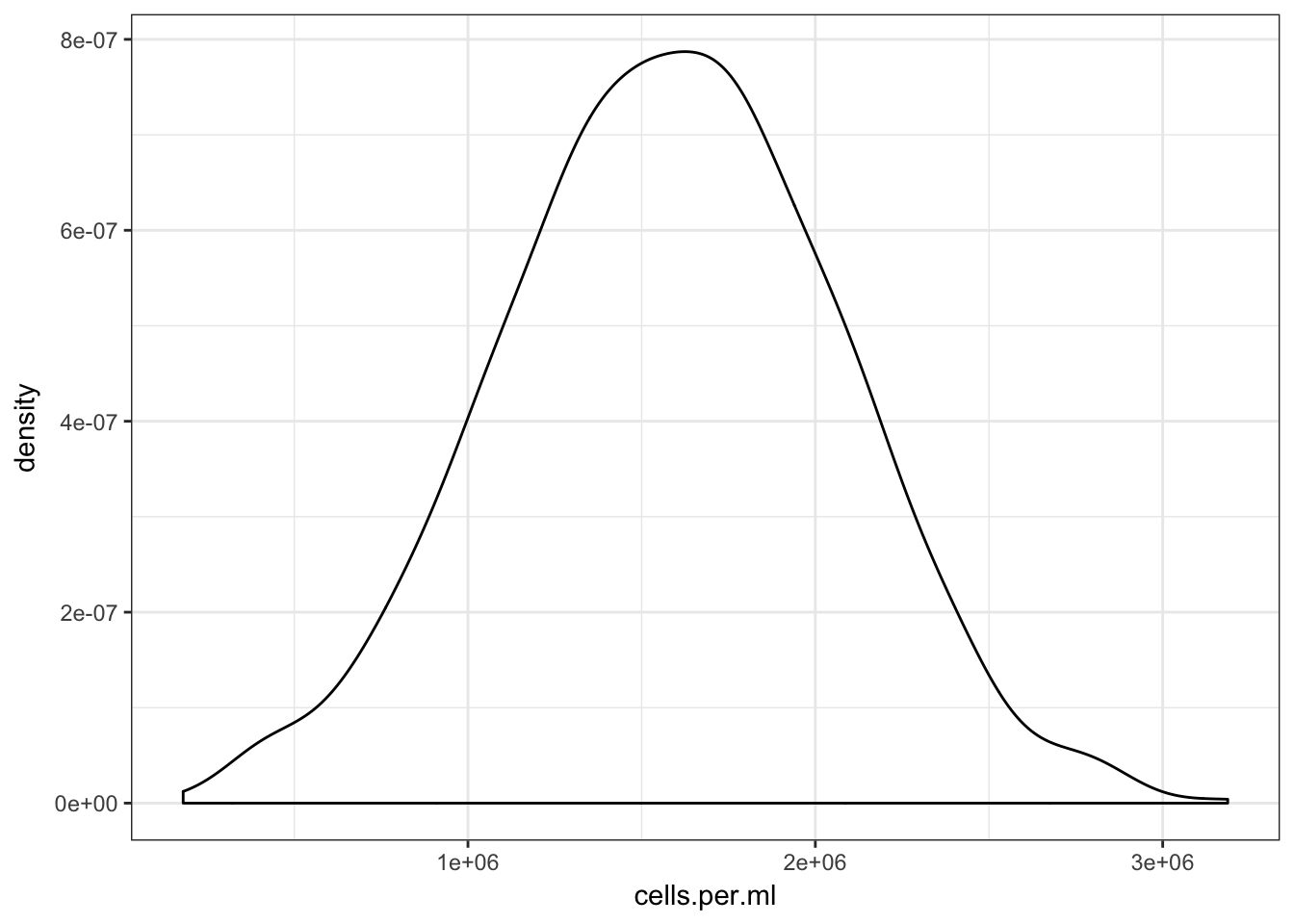
Now we can plot the distribution of the ratio of droplets with only 1 cell in them to the droplets with more than 1 cell in them.
ggplot(enframe(d, "iter", "Ratio"), aes(x=Ratio)) +
  geom_density() +
  theme_bw() +
  xlim(c(0, 10)) +
  xlab("Ratio of droplets with 1 cell / more than 1 cell")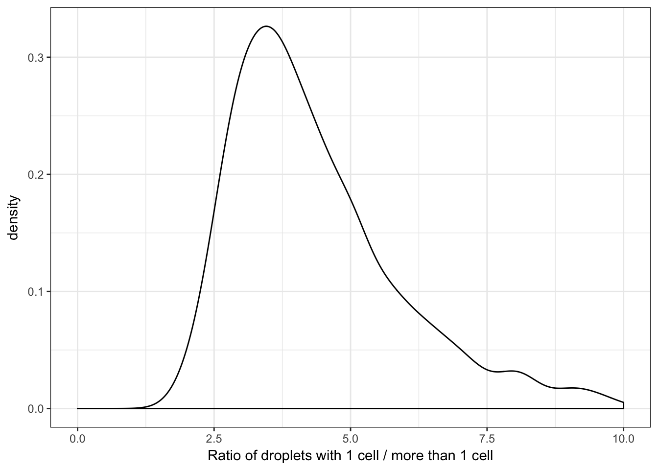
One thing to notice is that this distribution is not normally distributed. This is important and implies that the relation between the cells.per.ml and this ratio is non-linear.
We can also calculate some summary statistics for the distribution of this ratio, particularly it is useful to calculate the median and 95% probability region.
quantile(d, probs = c(0.025, 0.5, 0.975), na.rm = TRUE)## 2.5% 50% 97.5%
## 2.347455 4.078967 11.348473Bivariate Distributions
As a final point, my colleagues are also interested in the ratio of the fraction of droplets with only 1 cell in them to the fraction of droplets with zero cells in them as this ratio represents a measure of the efficiency of their method. If this ratio is too low then they are wasting space and energy making lots of empty droplets. We can actually visualize the uncertainty in both of these ratios as a bivariate distribution.
d <- data.frame(matrix(0, length(lambda), 2))
colnames(d) <- c("r1", "r2")
for (i in 1:length(lambda)){
  x <- dpois(j, lambda[i])
  d[i,"r1"] <- x[2]/(1-sum(x[c(1,2)]))
  d[i,"r2"] <- x[2]/x[1]
}
d %>%
  ggplot(aes(x = r1, y = r2)) +
  geom_density_2d() +
  theme_bw() +
  xlab("Ratio of droplets with 1 cell / more than 1 cell") +
  ylab("Ratio of droplets with 1 cell / zero cells")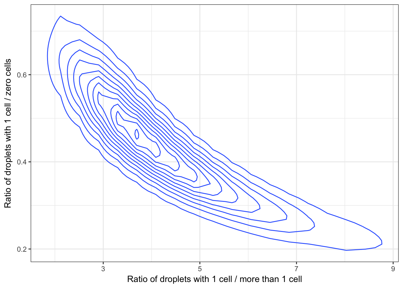
Ideally we would like to be in the top right portion of this plot where most of the droplets have 1 cell in them with few droplets with zero or more than 1 cell. However, ultimately there will be a trade off between the number of droplets with zero cells (efficiency) and the number off droplets with no more than 1 cell (specificity) and it is up to the researcher to determine what is reasonable for their applicaiton.