Fitting Non-Linear Growth Curves in R

A few months ago I offered to help a friend fit a bunch of microbial growth curves using R. When I was looking over possible solutions I was quite supprised by how little information was available online. Apart from the R package grofit (which after playing around with I decided seemed a little over-designed for my uses) I found very limited recources or code available. As a result of this I wanted to share a few functions I wrote to quickly fit non-linear growth models. I was specifically asked to help fit growth curves using the gompertz function and this is what I demonstrate below. I hope that this example gives some insight into how to fit non-linear models in R, beyond simply gompertz gorwth curves.

library(tidyverse)
set.seed(4)

To fit the gompertz model I use the nls (nonlinear least squares) function built into R. Its pretty straight forward however picking the correct starting values for the optimization was somewhat non-trivial. After a few attempts I found a way of defining the starting values that seemed to work for all the data I was given. The key idea is to use some simple and easy to compute approximation for each of the parameters of the model and use this as the starting value for the optimization.

The main function is fit.gompertz. This function returns the result of the nls function call. The function takes two arguments data and time which should be vectors of equal length giving the abundance and the times respectively for a given growth curve. The gompertz function I am fitting is the same one used by the package grofit, that is \[\text{data}\sim A e^{-e^{µ e/A(\lambda-\text{time}+1)}}\] where \(A\) defines the maximum of the curve, \(\mu\) defines the maximum slope, and \(\lambda\) is related to the lag-phase (e.g., the location of the maximum slope along the time axis). Note: this function assumes that the data/time vectors are ordered with respect to time (this is because of the way I use the diff function to pick starting values. )

fit.gompertz <- function(data, time){
  d <- data.frame(y=data, t=time)
  
  # Must have at least 3 datapoints at different times
  if (length(unique(d$t)) < 3) stop("too few data points to fit curve")
  
  # Pick starting values ###
  i <- which.max(diff(d$y))
  starting.values <- c(a=max(d$y), 
                       mu=max(diff(d$y))/(d[i+1,"t"]-d[i, "t"]), 
                       lambda=i)
  print("Starting Values for Optimization: ")
  print(starting.values)
  ##########################
  
  formula.gompertz <- "y~a*exp(-exp(mu*exp(1)/a*(lambda-t)+1))"
  nls(formula.gompertz, d, starting.values)
}

Now we are going to create some simulated data to test this on.

gompertz <- function(time, a, mu, lambda){
  y <- a*exp(-exp(mu*exp(1)/a*(lambda-time)+1))
  return(data.frame(time=time, y=y))
}

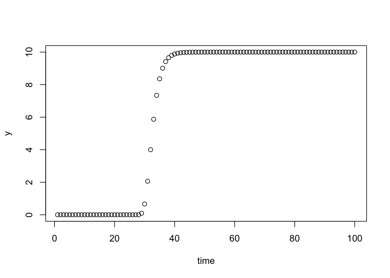
d <- gompertz(1:100, 10, 2, 30)
plot(d)

This is just the deterministic gompertz function. Now lets add some measurement noise

# Add some normal(0,0.5) noise centered around the deterministic signal
for(i in 1:nrow(d)) d[i,2] <- rnorm(1, d[i,2], 1)

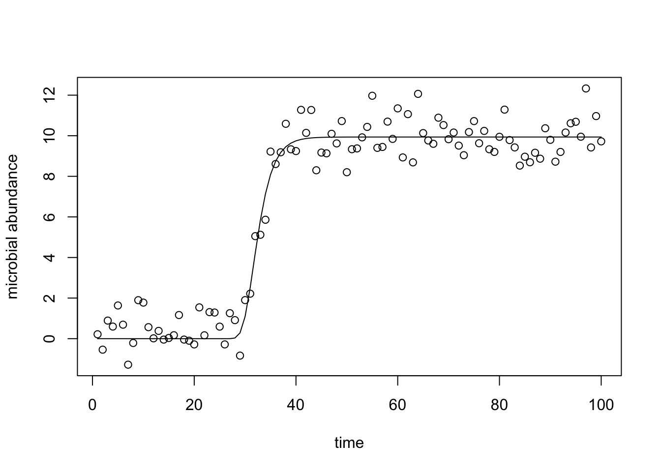
Now fit the noisy data and and plot the resulting fitted model.

(fit <- fit.gompertz(d$y, d$time))

## [1] "Starting Values for Optimization: "
##         a        mu    lambda 
## 12.330322  3.376417 63.000000

## Nonlinear regression model
##   model: y ~ a * exp(-exp(mu * exp(1)/a * (lambda - t) + 1))
##    data: d
##      a     mu lambda 
##  9.937  1.735 29.564 
##  residual sum-of-squares: 82.44
## 
## Number of iterations to convergence: 17 
## Achieved convergence tolerance: 2.223e-06

plot(d, ylab="microbial abundance")
lines(d$time, predict(fit))

One thing to note, if you find that the fit.gompertz function gives an error warning about a singular gradient: the problem is almost certanly that the starting values are far from the optimal and you should plot the data and estimate better values.

I also would suggest using the purrr::safely function to fit many curves at once. This is because the nls function often returns errors for poorly fit models and its a pain to have to keep excluding data-points/curves manually (easier to just collect the errors).

Below I create a “safe” version of the fit.gompertz function that collects errors rather than stopping evaluation.

safe.fit.gompertz <- safely(fit.gompertz)

To demonstrate how this works lets try it out on a growth curve with only 2 datapoints (something we know) will throw an error.

safe.fit.gompertz(c(1,2), c(19, 19))

## $result
## NULL
## 
## $error
## <simpleError in .f(...): too few data points to fit curve>

The new safe.fit.gompertz function returns a list with errors and results separated. This is particularly useful when used with purrr::map.

The other feature I found particularly useful was the AIC value for the fitted model. A low AIC is suggestive of poor model fit. In practice I found it useful to fit each growth curve and report the AIC value; then I would sort the fitted models by AIC and visually inspect the fitted models with the lowest AIC. This allowed me to quickly choose which growth curves were likely problematic so my friend could go back and collect those measurements again. This approached saved us a lot of time as there were hundreds-thousands of growth curves to analyze. Usefully, in R the AIC can be calculated by calling the function AIC directly on the fitted model object.

AIC(fit)

## [1] 272.4798

I hope this helps those that are trying to fit some non-linear models in R.